Keyword Analysis in Excel

by Marie Hoie, Senior Audit Data Analyst

Posted on February 20, 2020

When most people think of keyword analysis, they likely think of it in the context of search engine optimization: that is, which keywords or search phrases that bring visitors to websites. However, the applications of keyword analysis are not limited to marketing strategies. Within the audit world, keyword searches can be used to analyze text fields in an organization’s general ledger or other financial documents. Searching for particular keywords helps to identify certain types of activity that may need to be reviewed by auditors. This could include most commonly occurring keywords, keyword usage by employee, or unusual activities that an auditor shouldn’t expect to see in large volumes.

HeinfeldMeech uses Caseware IDEA data analysis software to perform our analytics test work. One of the software’s benefits is that it enables us to search our client’s audit files quickly and thoroughly for specific keywords and word variants. However, keyword analysis can still be performed in Excel with the proper set-up.

The steps below will enable you to perform a simple keyword analysis on a text column of a spreadsheet in Excel:

Step 1

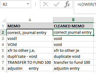
Determine which column to analyze for keywords. All cells in that column should be free of punctuation, excess spacing, and capitalization. Therefore, a new column must be created to clean the data from the original column’s cells using the formula below.

 [NOTE: be sure to change the cell reference (in red) to match your own spreadsheet]

=LOWER(TRIM(SUBSTITUTE(SUBSTITUTE(SUBSTITUTE(SUBSTITUTE(SUBSTITUTE(SUBSTITUTE(SUBSTITUTE(SUBSTITUTE(SUBSTITUTE(A2,”(“,” “),”)”,” “),”-“,””),”:”,””),”;”,””),”!”,””),”,”,””),”.”,””),”‘”,””)))

Step 2

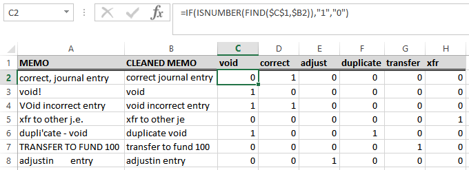
Add new columns for all keywords you’re interested in searching for within the data. Determine whether each keyword should be a whole word, a word root (e.g. “adjusting” vs. “adjust”), or a word abbreviation (e.g. “transfer” vs. “xfr”).

Enter those keywords as headers in the new columns, then enter the formula below into each cell of the keyword columns. This formula references each keyword column header and looks for that text within the cleaned data column. A “1” means the keyword occurs; a “0” means it does not occur.

 [NOTE: be sure to change the cell references (in red) to match your own spreadsheet]

=IF(ISNUMBER(FIND($C$1,$B2)),”1″,”0″)

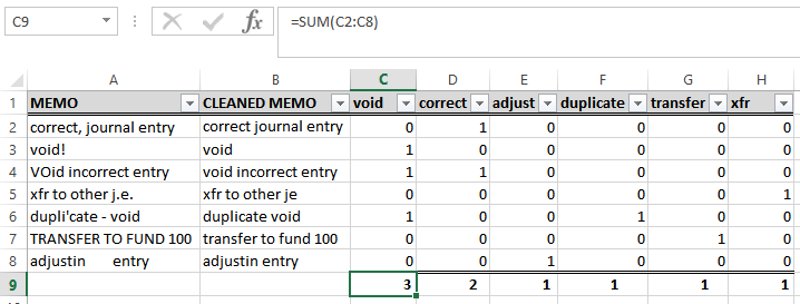
Step 3

The keyword columns should now be full of zeroes and ones indicating where each keyword occurs. However, the cells are not yet in a format that will enable them to be summed.

In order to generate the sums of occurrences for each keyword, the cells must first be reformatted via the following steps:

First, enter the number “1” into an unused cell in your spreadsheet. Copy the cell.

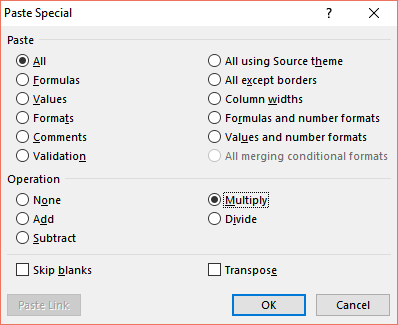
Then select the cells that need to be reformatted, then right-click inside the cells selection and click “Paste Special” (the words, not the arrow).

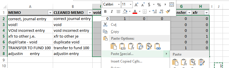
Next select “Multiply” from the Paste Special window and click OK.

The keyword cells are now in the correct format to be summed.